Kaldi Troubleshooting Head-to-Toe
Introduction
The following guide is for those who have already installed Kaldi, trained a GMM model, and trained a DNN model, but the final system isn’t performing well.
If you’re looking to get started with Kaldi, feel free to click on either of the above links and then come back to this guide as needed.
If you’re looking for a quick answer to a hyperparameter setting, check out this Kaldi Cheatsheet.
If you’d like a simple, easy to understand Kaldi recipe, you can check out the easy-kaldi GitHub repo. You probably won’t get state-of-the-art results with easy-kaldi, but you will hopefully be able to understand the pipeline.
Big Picture
The typical Kaldi training pipeline consists of the following four steps:
| Step | Dependencies |
|---|---|
| Train Monophones | pairs of <utterance, transcript> training data |
| Train Triphones | Monophone alignments |
| Train Speaker Adaptations | Triphone alignments |
| Train Deep Neural Network | Triphone + Speaker Adaptation alignments |
The first three steps all involve Gaussian Mixture Models and Hidden Markov Models (GMM-HMMs). So, even if you only care about the Deep Neural Network (DNN), you can’t avoid GMMs.
More importantly, you can’t just train those GMMs, generate the alignments for the deep neural network, and spend all your time tweaking neural net parameters in the hopes of getting a great model. You need to take the time to ensure that your GMMs are as high-performing as possible, or else all the parameter tweaking in the world won’t save your neural net. The GMMs are the foundation upon which your neural network is built, and you need to make sure you have a strong foundation. Otherwise you’re just building a house on sand.
The following document is a walk-through and troubleshooting guide for the entire training pipeline in Kaldi.
Problem Statement
Problem: You have a trained Kaldi system, but it performs poorly.
Once you have a working Automatic Speech Recognition (ASR) system built on Kaldi, your next step will be to improve that system’s performance. To be clear, by “ASR system”, I’m referring to the combination of the Acoustic Model and the Language Model.
Word Error Rates (WER) are the metric we most often use when evaluating a system’s performance, and WER must be interpreted as the combined performance of the two parts: (Acoustic Model and Language Model) – remember that. To improve WER as much as possible, you may need to address issues in both models. Nevertheless, isolated improvements to either model should lead to improvements in overall WER.
WER is the most important metric to optimize , but in the following we will focus on other metrics and data which represent only the Acoustic Model. We will troubleshoot starting from the last step of Kaldi training (i.e. the DNN), and work our way backwards to the first step (i.e. the Monophones).
Troubleshooting the Neural Network Acoustic Model
The first thing we need to do is identify the source of the problem: the Acoustic Model or the Language Model. It’s hard to troubleshoot the Language Model on it’s own, so we will start with the neural Acoustic Model. If after following this guide you conclude that the Acoustic Model is performing fine, then you should spend time on the Language Model (i.e. try training on new text data, train larger order N-grams, etc).
The Acoustic Model sends its output (i.e. phoneme predictions) to the Language Model, and then the Language Model tries to translate those predictions into words. A junk Acoustic Model will send junk predictions down the pipeline to the Language Model, and in the end you’ll get junk output from the Language Model.
Frame-Classification Accuracy
As mentioned above, WER is the most important metric for overall system performance. However, with regards to the neural Acoustic Model, frame-classification accuracy is the most relevant metric you can optimize. This metric tells you how well the Acoustic Model is able to assign a class label (i.e. phoneme ID) to a new slice of audio (i.e. audio frame). The Acoustic Model exists solely to perform this one task, and if the Acoustic Model is performing this task poorly the overall WER will be high.
To find data on frame-classification accuracy, we need to look at the relevant Kaldi log files: (1) compute_prob_train.*.log and (2) compute_prob_valid.*.log.
Here’s an example of what the contents of one of these log files could look like from an nnet2 model, using the Unix program cat:
$ cat log/compute_prob_valid.10.log
# nnet-compute-prob exp/nnet2_online/nnet_a/10.mdl ark:exp/nnet2_online/nnet_a/egs/valid_diagnostic.egs
# Started at Sun May  7 18:05:18 UTC 2019
#
nnet-compute-prob exp/nnet2_online/nnet_a/10.mdl ark:exp/nnet2_online/nnet_a/egs/valid_diagnostic.egs
LOG (nnet-compute-prob[5.2.110~1-1d137]:main():nnet-compute-prob.cc:91) Saw 4000 examples, average probability is -4.32658 and accuracy is 0.275 with total weight 4000
-4.32658
# Accounting: time=6 threads=1
# Ended (code 0) at Sun May  7 18:05:24 UTC 2019, elapsed time 6 seconds
These log files contain lines of the form accuracy is X, where X is the percent frame-classification error. The log file name contains the iteration number in training the neural net (e.g. compute_prob_train.10.log contains accuracy on the training data for the 10th iteration).
There are two important kinds of frame-classification accuracy: (1) the accuracy on the training set, and (2) the accuracy on a held-out validation set. The filename of the log contains information as to whether the statistics pertain to the training set or the validation set (i.e. compute_prob_train.*.log is the accuracy on the training set, and compute_prob_valid.*.log is the accuracy on the validation set).
These two accuracies give you very important information. Here is an example graph of these two metrics over time, where time is measured in iterations of backpropagation during training. We can see that on the training data, accuracy is reaching over 80%, but on the held-out validation data, the performance is actually getting worse over time, sinking towards 20% accuracy. This model has overfit the training data.
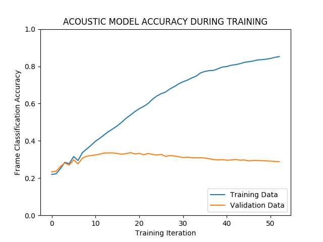
The data used to create this graph come from the relevant log files: (compute_prob_train.*.log and compute_prob_valid.*.log). The visualization scripts used to plot the data can be found here (format data) and here (plot data).
First, run the formatting script. It takes three args (1) the directory in which the compute.*.log files are saved, and (2) whether you’re using nnet2 vs nnet3, and (3) the filename of an output file which will then be used for plotting.
$ ./format_accuracy_for_plot.sh "/full/path/to/log/" "nnet3" "output_file.txt"Second, take the newly formatted data and plot it with Python.
$ python3 plot_accuracy.py -n 1 -t “My Awesome Title” -i "output_file.txt"There will be two lines plotted, one for the validation data and one for the training data. The flag -n is for number of tasks (because I also use the script for multi-task research). You just set number of tasks to one.
How to interpret frame-classification accuracy on training data?
Frame-classification accuracy on the training set (i.e. data from compute_prob_train.*.log) tells you how well your net is performing on the data it sees during training. If you make your neural net big enough and run enough training iterations (i.e. epochs), then you will get 100% accuracy on this data. This is a bad thing. When you get really high classification accuracy on the training set, this is typically a sign of overfitting. Your Acoustic Model has stopped “learning” patterns in speech, and started “memorizing” your data. Once you’ve overfit, your model is doing more table look-up than pattern recognition. So, getting 100% frame classification accuracy on your training data is a bad thing.
What to do about neural net overfitting on training data?
Two simple solutions: (1) Make the net smaller, and (2) don’t run so many epochs. There are many other, more complex solutions, but these two are good first steps.
When changing the size and architecture of the model, I’d suggest to first experiment with adjusting the number of hidden layers, and only afterwards experiment with the number of dimensions in each hidden layer. You should see larger increases or decreases in performance that way. To get an idea of what the code looks like for these parameters, check out an example of nnet3 code here or nnet2 code here.
How to interpret frame-classification accuracy on validation data?
The second metric from Acoustic Model training is frame-classification accuracy on a held-out validation set. You will find this information in the log files of the type: compute_prob_valid.*.log.
Frame-classification accuracy on the held-out validation set is the metric you want to optimize in DNN Acoustic Model training.
Frame-classification accuracy on the held-out validation set represents how well your Acoustic Model is able to classify data that it never saw before. There is no chance that the model ``memorized’’ this data.
Getting bad accuracy on validation data can mean two things: (1) there’s a problem with your data, and/or (2) there’s a problem with your model. If you’re using off-the-shelf code from Kaldi, you probably don’t have issues in your model. You might have to change the size of the model, but that’s all. What’s more often the issue is the data. You might have too little data, too noisy of data, or you might have mis-labeled data. Your mis-labeled data could mean that (1) the human transcriber did a bad job writing down all the correct words spoken in the audio, (2) the phonetic dictionary has incorrect pronunciations for words, or (3) the GMM-HMM system did a bad job aligning data to monophones or triphones.
If your data and labels are wrong, then your neural model won’t be able to learn anything. Think of the case where you’re training a neural net to identify pictures of dogs and cats, but you had a bad annotator who labeled a bunch of dogs as if they were cats. Your system won’t be able to learn what a dog looks like, because the training data was wrong in the first place. In Kaldi (and hybrid DNN-HMM speech recognition in general) we don’t have a human annotator labeling each chunk of audio as belonging to a certain phoneme. Rather, we use a GMM-HMM system to produce those annotations via forced alignment.
In what follows we’re going to talk about troubleshooting the GMMs systems you use in Kaldi to generate those alignments (i.e. monophones / triphones / LDA + MLLT / SAT).
Troubleshooting your GMM-HMMs
Now that we know why GMMs are so important, let’s find out if they’re working correctly. There’s a few important metrics and datapoints to help you gauge how well your GMMs are performing:
| Data Points | From where? |
|---|---|
| Alignments | training data |
| Transcripts | decoded test data |
WER |
decoded test data |
These three sources of information all tell us how a given GMM model is performing, and it’s important to know where each piece comes from. The alignments, transcripts, and WER all are generated as outputs from the GMM-HMM training pipeline. Whether you’re training monophones or triphones with Speaker Adaptive Training (SAT), you will have to go through these same three steps, and as a result you will produce outputs which can be inspected.
Where these GMM-HMM performance metrics come from:
| Step | Outputs |
|---|---|
| Alignment | Alignments |
| Training | GMM-HMMs |
| Decoding | WER + Transcripts |
It’s hard to directly inspect GMM-HMMs, which is why we make use of the outputs of the training and testing phases (WER / transcripts / alignments). The outputs listed above will be produced individually for each model you train, so you can see how the models (e.g. monophones vs. triphones) compare to each other. You can find the code corresponding to each of these three steps in the wsj/s5/run.sh file at the following locations.
I chose to reference this run.sh from the Wall Street Journal recipe (i.e. called wsj in Kaldi) because all other examples in Kaldi link back to wsj. This is the root of all Kaldi example recipes (so-called egs).
Training Steps in wsj/s5/run.sh
To the left is the line number, in the center is the actual code, and to the right is my comment on what the line refers to.
97   steps/train_mono.sh --boost-silence 1.25 --nj 10 --cmd "$train_cmd" \                  <-- mono
        data/train_si84_2kshort data/lang_nosp exp/mono0a

116  steps/train_deltas.sh --boost-silence 1.25 --cmd "$train_cmd" 2000 10000 \             <--  tri
        data/train_si84_half data/lang_nosp exp/mono0a_ali exp/tri1

157  steps/train_lda_mllt.sh --cmd "$train_cmd" \                                <--  tri + LDA+MLLT
        --splice-opts "--left-context=3 --right-context=3" 2500 15000 \
        data/train_si84 data/lang_nosp exp/tri1_ali_si84 exp/tri2b

211  steps/train_sat.sh --cmd "$train_cmd" 4200 40000 \                    <--  tri + LDA+MLLT + SAT
        data/train_si284 data/lang_nosp exp/tri2b_ali_si284 exp/tri3b
Alignment Steps in wsj/s5/run.sh
N.B. there is no explicit alignment of the tri + LDA+MLLT + SAT model in wsj/s5/run.sh
113  steps/align_si.sh --boost-silence 1.25 --nj 10 --cmd "$train_cmd" \                    <-- mono
        data/train_si84_half data/lang_nosp exp/mono0a exp/mono0a_ali

154  steps/align_si.sh --nj 10 --cmd "$train_cmd" \                                          <-- tri
        data/train_si84 data/lang_nosp exp/tri1 exp/tri1_ali_si84

208  steps/align_si.sh --nj 10 --cmd "$train_cmd" \                               <-- tri + LDA+MLLT                                                                                       	  data/train_si284 data/lang_nosp exp/tri2b exp/tri2b_ali_si284
Decoding Steps in wsj/s5/run.sh
103  steps/decode.sh --nj 8 --cmd "$decode_cmd" exp/mono0a/graph_nosp_tgpr \               <--  mono
        data/test_eval92 exp/mono0a/decode_nosp_tgpr_eval92

126  steps/decode.sh --nj $nspk --cmd "$decode_cmd" exp/tri1/graph_nosp_tgpr \              <--  tri
        data/test_${data} exp/tri1/decode_nosp_tgpr_${data}

167  steps/decode.sh --nj ${nspk} --cmd "$decode_cmd" exp/tri2b/graph_nosp_tgpr \ <-- tri + LDA+MLLT
        data/test_${data} exp/tri2b/decode_nosp_tgpr_${data}

230  steps/decode_fmllr.sh --nj ${nspk} --cmd "$decode_cmd" \              <--  tri + LDA+MLLT + SAT
        exp/tri3b/graph_nosp_tgpr data/test_${data} \
        exp/tri3b/decode_nosp_tgpr_${data}
Interpreting WER
WER are a measure of the combined performance of the Acoustic Model + Language Model, so we have to take them with a grain of salt when we use them to talk about the Acoustic Model alone. If the Acoustic Model is performing badly, but your Language Model is well suited to your data, you may still get good WER.
The decoding phase produces WER, which help you quickly gauge the performance of your model. For example, you might see something like the following:
| Step | WER |
|---|---|
| Monophones | 10% |
| Triphones | 9% |
| Triphones + LDA + MLLT | 7% |
| Triphones + LDA + MLLT + SAT | 82% |
| Train Deep Neural Network | 80% |
In this case, you know that something went wrong between stage triphones + LDA + MLLT and stage triphones + LDA + MLLT + SAT, because all previous models were doing just fine. We don’t have to worry about trying to debug those previous models, because errors are propagated only from the most recent model. In the example shown above, you don’t have to waste time looking at your monophones or vanilla triphones (i.e. delta+delta triphones in Kaldi-speak), because they couldn’t have been responsible.
The WER for your models can be found in the following locations within your experiment directory (i.e. exp):
exp/mono0a/decode_*/wer_*        <-- monophones

exp/tri1/decode_*/wer_*          <--  triphones

exp/tri2b/decode_*/wer_*         <--  triphones + LDA + MLLT

exp/tri3b/decode_*/wer_*         <--  triphones + LDA + MLLT + SAT
Here’s an example of how WER are reported:
$ cat /tri2b/decode_test_clean/wer_8_0.0
compute-wer --text --mode=present ark:exp/tri2b/decode_test_clean/scoring/test.txt ark,p:-
%`WER` 7.82 [ 4109 / 52576, 692 ins, 314 del, 3103 sub ]
%SER 60.04 [ 1573 / 2620 ]
Scored 2620 sentences, 0 not present in hyp
As you can see, we get more info than just the WER. We also get the Sentence Error Rate (SER) and importantly, we get info on the size of the test set. Here we see that 2620 sentences were in this test set.
We also get information on how many times the system failed during decoding: 0 not present in hyp. hyp stands for hypothesis, and if that number is greater than 0, it means that the model was unable to generate a hypothesis transcript for atleast one utterance (i.e. decoding failed). Failed decoding may happen if the decoding beam is too small or if the audio is exceptionally noisy.
Interpreting Alignments
The alignment logs are found in exp/*_ali/log/ali.*.gz
After WER, the second place we can troubleshoot a model is by looking at the alignments that were used to train that model. If the alignments are bad, then the resulting model will perform poorly.
As we saw in the Big Picture, at each step information from the previous model (e.g. monophones) is passed to the next model (e.g. triphones) via alignments. As such, it’s important that you’re sure that at each step the information passed downstream is accurate. Before we jump into the alignment files, let’s talk a little about what alignments are in the first place.
You can think of alignments as audio with time-stamps, where the time-stamps correspond to the sounds that were spoken in that audio (i.e. phonemes – sometimes called senomes, which may also be graphemes or just characters).
As you can see in the image below, there is some audio utterance (shown on top via waveform), and we have some text utterance associated with that audio, and after alignment we end up with the bottom row (alignments of individual phonemes to slices of audio).
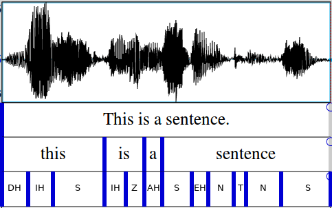
This alignment corresponds to a monophone model, because each phoneme (i.e. linguistic speech sound) is modeled by only one unit. For example, you can see that there are multiple instances of the sound S, and they are all coded exactly the same (i.e. S). Each instance of S is actually acoustically different from the others, because each instance has its own neighboring sounds which affect it: this is called the co-articulation affect.
Triphone models take this co-articulation effect into account by modeling phonemes based on context. The triphone alignment would look something more like this:
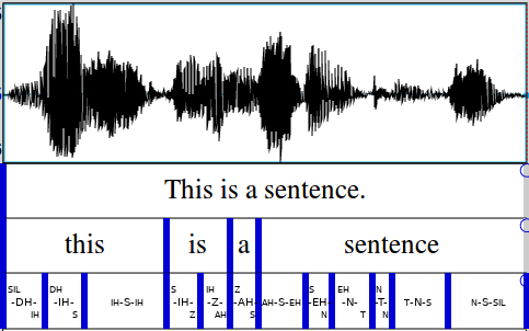
The sounds are now encoded with their surrounding context. For example, IH-Z-AH represents the sound Z which is preceded by the sound IH and followed by the sound AH.
Triphone alignments are more complicated than monophones. This extra complication allows for the modeling of more nuanced phonetic details. In the monophone alignments we see that the S from “this” and the ‘S’ from “is” are modeled as the same sound. However, in reality these two S sounds are acoustically very different, because they have different neighboring phonemes. The monophone alignments lose this distinction, but the triphones capture it. These two ‘S’s are modeled as separate units in the triphone alignments.
Triphone models take into account (a) the central phoneme of interest, (b) the phoneme to the immediate left, and (c) the phoneme to the immediate right. As such, triphones take into account three phonemes (this is where the word “triphone” comes).
Each step in the training pipeline (monophone, triphone, triphone + adaptation) generates its own set of alignments, and these alignments can be found in the following locations:
exp/mono0a_ali/ali.*.gz          <--  monophones

exp/tri1_ali/ali.*.gz            <--  triphones

exp/tri2b_ali/ali.*.gz           <--  triphones + LDA + MLLT

exp/tri3b_ali/ali.*.gz           <--  triphones + LDA + MLLT + SAT
Direct inspection of alignments
We can directly inspect these alignments with Kaldi tools.
What we would like to see from these tools are the following: (1) all the words spoken in the utterance are found in the alignment, and (2) the words and phonemes are appropriately spaced in time. For both of these, the file get_train_ctm.sh will be particularly helpful because it shows the words in the utterance along with their time-stamps.
You should be able to see if the transcript contains missing words, extra words, or if the timing is off. I’d suggest you look at an utterance from the ctm file and listen to the audio at the same time. This way you can compare what you hear to what the system is producing.
Here’s how you can pull out the word-level alignments from one file (e.g. ID_354.wav):
# create the ctm file
$ steps/get_train_ctm.sh data/train/ data/lang exp/tri_ali/

# pull out one utt from ctm file
$ grep ID_354 exp/tri_ali/ctm
ID_354 1 0.270 0.450 the
ID_354 1 0.720 0.420 dog
ID_354 1 1.140 0.330 ran
ID_354 1 1.470 0.510 home
These word-level alignments look good, but we can even get a finer-grained look at alignments by inspecting the phoneme-level alignments with show-alignments.cc.
$ show-alignments data/lang/phones.txt exp/tri1_ali/final.mdl ark:"gunzip -c ali.1.gz |" | grep "ID_354"
ID_354 [ 4 1 1 1 16 18 ] [ 21958 21957 22115 22115 ] [ 39928 40076 40075 40296 40295 40295 40295 40295 ] [ 44894 44893 45211 45211 ][ 4 16 18 ] [ 28226 28268 28267 28267 28267 28267 28267 28267 28314 28313 ] [ 34762 34846 34914 ] [ 63728 63918 63958 ] [ 4 1 18 ]
ID_354  SIL       DH      AH1  D              AA    G        R      AE      N HH               OW         M                 SIL
I just made up the alignment above to fit nicely in this guide, but the structure is identical to what show-alignments.cc will produce. There are two lines produced, which both begin with the utterance ID of the audio file we’re interested in (e.g. ID_354). The first line has a bunch of numbers and square brackets separated by spaces, where the individual numbers correspond to sub-parts of phonemes (i.e. individual states of the HMM-GMM), and the brackets show you where the phonemes themselves start and end. You should find two square brackets ([ and ]) for each phoneme in the utterance. A number is repeated as many times as the model passed through that HMM state. Phonemes which take up more time in the audio itself will have more numbers within their brackets.
As you can see in the output from show-alignments.cc, silence (i.e. SIL) is made explicit at the beginning and end of each utterance. The alignment procedure assumes that there is some silence at the beginning and end of the audio file. If you don’t have silence in the audio, your alignment procedure will still proceed as if there really is silence in the audio. As such, your GMM-HMM model will ``find’’ silence in the audio, even if it isn’t there, and estimate the acoustic properties of silence based on speech instead – this is bad. You should try to have silence at the beginning and end of your audio files.
A very nice thing about inspecting alignments is that they are independent of the Language Model. That is, only the phonetic dictionary and the training transcripts are used to generate the alignments.
You can get an idea of which words are causing alignment issues by looking into the log flies from alignment (i.e. the acc.*.log files, which accumulate stats from alignments) as such. When an alignment fails, you will find “No alignment for utterance” and then the utterance ID in these acc.*.log files. To find all issues in your triphones, simply grep as such:
$ grep -r "No alignment" exp/tri*/log/acc.*.logThis usually means either there’s a mis-match between the audio and the transcript, or the audio is really noisy.
$ grep -r "gmm-align-compiled.* errors on " exp/tri*_ali/log/align_pass*.logFor statistics on the phonemes you trained and where they’re located, take a look the analyze_alignments.log files which you find in your alignment directories (e.g. exp/tri*_ali/log/analyze_alignments.log).
Interpreting the Decoding Transcripts from Test Data
Another place that we can evaluate the performance of a GMM-HMM model is by inspecting the transcripts that it produced at decoding time on the test data. These results reflect both the Acoustic Model, the Language Model, and the decoding time parameters.
You can find the decoding output in the following log files:
exp/mono0a/decode_*/scoring/log/best_path.*.log <-- monophones

exp/tri1/decode_*/scoring/log/best_path.*.log   <-- triphones

exp/tri2b/decode_*/scoring/log/best_path.*.log  <-- triphones + LDA + MLLT

exp/tri3b/decode_*/scoring/log/best_path.*.log  <-- triphones + LDA + MLLT + SAT
If we take a look into one of those log files, we will see something like this:
$ head -25 tri2a/decode_test/scoring/log/best_path.10.0.0.log | tail
ID-0004 NUMBERED DEN A FRESH NELLIE IS WAITING ON YOU GOOD NIGHT HUSBAND
LOG (lattice-best-path[5.2.110~1-1d137]:main():lattice-best-path.cc:99) For utterance ID-0005, best cost 204.174 + 3882.34 = 4086.51 over 962 frames.
ID-0005 THE MUSIC CAME NEARER AND HE RECALLED THE WORDS THE WORDS OF SHELLEY'S FRAGMENT UPON THE MOON WANDERING COMPANIONLESS PALE FOR WEARINESS
LOG (lattice-best-path[5.2.110~1-1d137]:main():lattice-best-path.cc:99) For utterance ID-0006, best cost 235.088 + 4450.84 = 4685.93 over 1054 frames.
ID-0006 THE DULL LIGHT FELL MORE FAINTLY UPON THE PAGE WHERE ON ANOTHER EQUATION BEGAN TO UNFOLD ITSELF SLOWLY AND TO SPREAD ABROAD ITS WIDENING TALE
LOG (lattice-best-path[5.2.110~1-1d137]:main():lattice-best-path.cc:99) For utterance ID-0007, best cost 90.7232 + 1771.01 = 1861.73 over 426 frames.
ID-0007 A COLD LUCID IN DIFFERENCE OR REINED IN HIS SOUL
LOG (lattice-best-path[5.2.110~1-1d137]:main():lattice-best-path.cc:99) For utterance ID-0008, best cost 136.785 + 2868.84 = 3005.63 over 671 frames.
The best_path in the filename best_path.10.0.0.log means that the output represents the 1-best path through the decoding lattice for each utterance. This is very useful, because this shows you how the model is performing at test-time, and you can spot errors and biases here more easily.
The first few lines are logging data, and the lines in all caps are the model’s prediction on some testing data. These lines show (1) the utterance ID (e.g. ID-0007), and (2) the prediction of the model for that utterance (e.g. A COLD LUCID IN DIFFERENCE OR REINED IN HIS SOUL). It is good to listen to the audio file and look at the corresponding output to identify errors.
Sometimes you can even see if the errors stem from the Acoustic Model or from the Language Model (e.g. the model predicted IN DIFFERENCE instead of INDIFFERENCE, which is a Language Model problem given that both options are acoustically identical).
What next for Acoustic Model troubleshooting?
If at this point you’ve run all the inspections above, your GMM-HMM model should perform well and your alignments should look good. What to do if you’re still having issues in training a good neural net?
Well, as mentioned above, if you’re overfitting your training data, then try to reduce the size of the model as well as the number of epochs you run. At this point you might need to do some hyper-parameter searching within the suggestions I provide below as a cheat-sheet. Try to identify consistent problems in the output of the combined model (Language Model + Acoustic Model).
Language Model
The Language Model (LM) is indeed very important for WER. The LM encodes (a) which words are possible, (b) which words are impossible, and (c) how probable each possible word is. A word may only be decoded if it occurs in the vocabulary of the Language Model. Any word that does not occur in the vocabulary is an Out-Of-Vocabulary (OOV) word. The Language Model contains a probability for each word and word sequence.
The LM you use in your application and the LM you use at test time to not need to be the same. However, if you’re optimizing WER at test-time by adjusting Language Model parameters, it isn’t guaranteed that improvements will transfer to inference with a new LM.
Notes on the Language Model you use at Test-Time
Improvements in WER which come from Acoustic Model parameter changes should generalize across Language Models. For example, if you find that for a bi-gram Language Model a 5-layer neural net Acoustic Model works better than a 6-layer net, you should expect that (for your data), a 5-layer Acoustic Model will beat out a 6-layer net, regardless of the n-gram order of the Language Model.
Conclusion
In short, when you’re troubleshooting your Kaldi system, first look at the training statistics for your Deep Neural Network Acoustic Model. Then, look at the training, alignment, and decoding stats of your GMM-HMMs. If all those data look good, then try training a Language Model more suited for your use-case.
If you still are running into issues, look on kaldi-help to see if someone else has had your problem (often they have). As far as I know, kaldi-help is the only forum for these kinds of questions. Unfortunately, the atmosphere on kaldi-help can be unwelcoming to newcomers. If you post a question and get a critical response, don’t let it upset you. The forum can be un-welcoming, and it has nothing to do with you or your abilities to do good ASR! I was afraid to post on kaldi-help for a long time because of this atmosphere, and indeed my first post was not received kindly. Alternatively, you can post questions here on my blog. However, the community here is not as large as kaldi-help.
I hope this was helpful, and happy Kaldi-ing!
Let me know if you have comments or suggestions and you can always leave a comment below.