A TensorFlow Tutorial: Email Classification

This code/post was written in conjunction with Michael Capizzi. Sections of the original code on which this is based were written with Joe Meyer.

Update: November 2, 2017 - New script for raw text feature extraction read_corpus.py

Update: March 8, 2017 - Now supports TensorFlow 1.0

Quick Start

You can get the code and data discussed in this post (as well as presentation slides from the Tucson Data Science Meetup) by cloning the following repo:

git clone https://github.com/JRMeyer/tensorflow-tutorial.git
cd tensorflow-tutorial

Dependencies

sudo apt-get install python3-pip
sudo pip3 install -r requirements.txt
sudo apt-get install python3-tk # for some reason won't work with pip3

Once you have the code and data, you can run a training session and get some output with the following:

tensorflow-tutorial$ python3 logistic_regression_train.py 
loading training data
loading test data
I tensorflow/core/common_runtime/local_device.cc:40] Local device intra op parallelism threads: 4
I tensorflow/core/common_runtime/direct_session.cc:58] Direct session inter op parallelism threads: 4
step 0, training accuracy 0.465897
step 0, cost 256.736
step 0, change in cost 256.736
         .
         .
         .

Introduction

This tutorial is meant for those who want to get to know the Flow of TensorFlow. Ideally, you already know some of the Tensor of TensorFlow. That is, in this tutorial we aren’t going to go deep into any of the linear algebra, calculus, and statistics which are used in machine learning.

Don’t worry though, if you don’t have that background you should still be able to follow this tutorial. If you’re interested in learning more about the math, there’s a ton of good places to get an introduction to the algorithms used in machine learning. This tutorial from Stanford University about artificial neural nets is especially good. We’re going to be using a simple logistic regression classifier here, but many of the concepts are the same.

Email Classification

To ground this tutorial in some real-world application, we decided to use a common beginner problem from Natural Language Processing (NLP): email classification. The idea is simple - given an email you’ve never seen before, determine whether or not that email is Spam or not (aka Ham).

For us humans, this is a pretty easy thing to do. If you open an email and see the words “Nigerian prince” or “weight-loss magic”, you don’t need to read the rest of the email because you already know it’s Spam.

While this task is easy for humans, it’s much harder to write a program that can correctly classify an email as Spam or Ham. You could collect a list of words you think are highly correlated with Spam emails, give that list to the computer, and tell the computer to check every email for those words. If the computer finds a word from the list in an email, then that email gets classified as Spam. If the computer did not find any of those words in an email, then the email gets classified as Ham.

Sadly, this simple approach doesn’t work well in practice. There’s lots of Spam words you will miss, and some of the Spam words in your list will also occur in regular, Ham emails. Not only will this approach work poorly, it will take you a long time to compose a good list of Spam words by hand. So, why don’t we do something a little smarter by using machine learning? Instead of telling the program which words we think are important, let’s let the program learn which words are actually important.

To tackle this problem, we start with a collection of sample emails (i.e. a text corpus). In this corpus, each email has already been labeled as Spam or Ham. Since we are making use of these labels in the training phase, this is a supervised learning task. This is called supervised learning because we are (in a sense) supervising the program as it learns what Spam emails look like and what Ham email look like.

During the training phase, we present these emails and their labels to the program. For each email, the program says whether it thought the email was Spam or Ham. After the program makes a prediction, we tell the program what the label of the email actually was. The program then changes its configuration so as to make a better prediction the next time around. This process is done iteratively until either the program can’t do any better or we get impatient and just tell the program to stop.

On to the Script

The beginning of our script starts with importing a few needed dependencies (Python packages and modules). If you want to see where these packages get used, just do a CTRL+F search for them in the script. If you want to learn what the packages are, just do a Google search for them.

################
### PREAMBLE ###
################

from __future__ import division
import tensorflow as tf
import numpy as np
import tarfile
import os
import matplotlib.pyplot as plt
import time

Next, we have some code for importing the data for our Spam and Ham emails. For the sake of this tutorial, we have pre-processed the emails to be in an easy to work with format.

The X-matrices (i.e. feature matrices) have the shape (number of rows, number of columns). Each row represents an email, and each column represents a word. Each cell in the matrix contains an interger between 0 and infinity (i.e. \(\mathbb{N}\)) which is the count of how many times a given word occured in a given email.

	great	dog	pill	\(\cdots\)
email_001	0	1	0	\(\cdots\)
email_002	3	0	5	\(\cdots\)
email_003	0	0	0	\(\cdots\)
\(\vdots\)	\(\vdots\)	\(\vdots\)	\(\vdots\)	\(\ddots\)

Similarly, we have a matrix which holds the labels for the our data. In this case, the matrix has two columns, one for Spam and one for Ham. There can only be a 1 or a 0 in each cell, where 1 means that column is the correct label for the email. Like in the feature matrix, each row in the matrix represents an email.

	Spam	Ham
email_001	0	1
email_002	1	0
email_003	1	0
\(\vdots\)	\(\vdots\)	\(\vdots\)

In these illustrations the matrices have row and column headers, but the actual matrices we feed into TensorFlow have none.

The import_data() function first checks if the data directory “data/” exists in your current working directory or not. If it doesn’t exist, the code tries to unzip the tarred data from the file “data.tar.gz”, which is expected to be in your current working directory.

You need to have either the “data/” directory or the tarred file “data.tar.gz” in your working directory for the script to work.

###################
### IMPORT DATA ###
###################

def csv_to_numpy_array(filePath, delimiter):
    return np.genfromtxt(filePath, delimiter=delimiter, dtype=None)

def import_data():
    if "data" not in os.listdir(os.getcwd()):
        # Untar directory of data if we haven't already
        tarObject = tarfile.open("data.tar.gz")
        tarObject.extractall()
        tarObject.close()
        print("Extracted tar to current directory")
    else:
        # we've already extracted the files
        pass

    print("loading training data")
    trainX = csv_to_numpy_array("data/trainX.csv", delimiter="\t")
    trainY = csv_to_numpy_array("data/trainY.csv", delimiter="\t")
    print("loading test data")
    testX = csv_to_numpy_array("data/testX.csv", delimiter="\t")
    testY = csv_to_numpy_array("data/testY.csv", delimiter="\t")
    return trainX,trainY,testX,testY

trainX,trainY,testX,testY = import_data()

Now that we can load in the data, let’s move on to the code that sets our global parameters. These are values that are either (a) specific to the data set or (b) specific to the training procedure. Practically speaking, if you’re using the provided email data set, you will only be interested in adjusting the training session parameters.

#########################
### GLOBAL PARAMETERS ###
#########################

# DATA SET PARAMETERS
# Get our dimensions for our different variables and placeholders:
# numFeatures = the number of words extracted from each email
numFeatures = trainX.shape[1]
# numLabels = number of classes we are predicting (here just 2: Ham or Spam)
numLabels = trainY.shape[1]

# TRAINING SESSION PARAMETERS
# number of times we iterate through training data
# tensorboard shows that accuracy plateaus at ~25k epochs
numEpochs = 27000
# a smarter learning rate for gradientOptimizer
learningRate = tf.train.exponential_decay(learning_rate=0.0008,
                                          global_step= 1,
                                          decay_steps=trainX.shape[0],
                                          decay_rate= 0.95,
                                          staircase=True)

TensorFlow Placeholders

Next we have a block of code for defining our TensorFlow placeholders. These placeholders will hold our email data (both the features and label matrices), and help pass them along to different parts of the algorithm. You can think of placeholders as empty shells (i.e. empty tensors) into which we insert our data. As such, when we define the placeholders we need to give them shapes which correspond to the shape of our data.

The way TensorFlow allows us to insert data into these placeholders is by “feeding” the placeholders the data via a “feed_dict”. You if you do a CTRL+F search for “feed” you will see that this happening in the actual training step.

This is a nice feature of TensorFlow because we can create an algorithm which accepts data and knows something about the shape of the data while still being agnostic about the amount of data going in. This means that when we insert “batches” of data in training, we can easily adjust how many examples we train on in a single step without changing the entire algorithm.

In TensorFlow terms, we build the computation graph and then insert data as we wish. This keeps a clean division between the computations of our algoritm and the data we’re doing the computations on.

####################
### PLACEHOLDERS ###
####################

# X = X-matrix / feature-matrix / data-matrix... It's a tensor to hold our email
# data. 'None' here means that we can hold any number of emails
X = tf.placeholder(tf.float32, [None, numFeatures])
# yGold = Y-matrix / label-matrix / labels... This will be our correct answers
# matrix. Every row has either [1,0] for SPAM or [0,1] for HAM. 'None' here 
# means that we can hold any number of emails
yGold = tf.placeholder(tf.float32, [None, numLabels])

TensorFlow Variables

Next, we define some TensorFlow variables as our parameters. These variables will hold the weights and biases of our logistic regression and they will be continually updated during training. Unlike the immutable TensorFlow constants, TensorFlow variables can change their values within a session.

This is essential for any optimization algorithm to work (we will use gradient descent). These variables are the objects which define the structure of our regression model, and we can save them after they’ve been trained so we can reuse them later.

Variables, like all data in TensorFlow, are represented as tensors. However, unlike our placeholders above which are essentially empty shells waiting to be fed data, TensorFlow variables need to be initialized with values.

That’s why in the code below which initializes the variables, we use tf.random_normal to sample from a normal distribution to fill a tensor of shape “shape” with random values. Both our weights and bias term are initialized randomly and updated during training.

#################
### VARIABLES ###
#################

# Values are randomly sampled from a Gaussian with a standard deviation of:
#     sqrt(6 / (numInputNodes + numOutputNodes + 1))

weights = tf.Variable(tf.random_normal([numFeatures,numLabels],
                                       mean=0,
                                       stddev=(np.sqrt(6/numFeatures+
                                                         numLabels+1)),
                                       name="weights"))

bias = tf.Variable(tf.random_normal([1,numLabels],
                                    mean=0,
                                    stddev=(np.sqrt(6/numFeatures+numLabels+1)),
                                    name="bias"))

TensorFlow Ops

Up until this point, we have defined the different tensors which will hold important information. Specifically, we have defined (1) the tensors which hold the email data (feature and label matrices) as well as (2) the tensors which hold our regression weights and biases.

Now we will switch gears to define the computations which will act upon those tensors. In TensorFlow terms, these computations are called operations (or “ops” for short). These ops will be the nodes in our computational graph. Ops take tensors as input and give back tensors as output.

In the illustration below, the green nodes represent our TensorFlow placeholders (holding features and labels), the blue nodes represent our TensorFlow variables (holding weights and biases), and the pink nodes represent our TensorFlow Ops (operations on our tensors).

logistic-regression

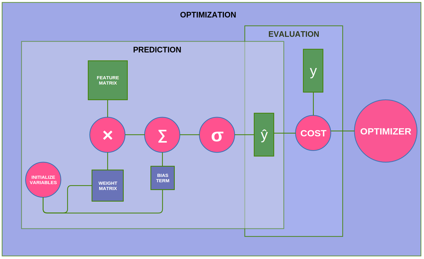
We will start with the operations involved in the prediction phase (i.e. the logistic regression itself). First, we need to initialize our weights and biases with random values via a TensorFlow Op. TensorFlow has a special built in Op for just this, since this is a step you will most likely have to perform everytime you use TensorFlow. Like all our other Ops, this Initialization Op will become a node in our computational graph, and when we put the graph into a session, then the Op will run and create the variables.

Next, we have our ops which define the logistic regression function. Logisitic regression is typically thought of as a single equation, (i.e. \(\mathbf{\hat{y}} = sig(\mathbf{WX} + \mathbf{b})\)), but for the sake of clarity we have broken it into its three main components (1) a weight times features operation, (2) a summation of the weighted features and a bias term, and (3) the application of a sigmoid function. As such, you will find these components defined as three separate ops below.

######################
### PREDICTION OPS ###
######################

# INITIALIZE our weights and biases
init_OP = tf.initialize_all_variables()

# PREDICTION ALGORITHM i.e. FEEDFORWARD ALGORITHM
apply_weights_OP = tf.matmul(X, weights, name="apply_weights")
add_bias_OP = tf.add(apply_weights_OP, bias, name="add_bias") 
activation_OP = tf.nn.sigmoid(add_bias_OP, name="activation")

Next we define our cost operation (i.e. Mean Squared Error). For this, we use TensorFlow’s built in L2 Loss function, \(\frac{1}{2} \sum_{i=1}^{N} (\mathbf{\hat{y}_i}-\mathbf{y_i})^2\).

#####################
### EVALUATION OP ###
#####################

# COST FUNCTION i.e. MEAN SQUARED ERROR
cost_OP = tf.nn.l2_loss(activation_OP-yGold, name="squared_error_cost")

Next, we define the function to optimize our cost function. We are using gradient descent, which TensorFlow has a built in op for.

#######################
### OPTIMIZATION OP ###
#######################

# OPTIMIZATION ALGORITHM i.e. GRADIENT DESCENT
training_OP = tf.train.GradientDescentOptimizer(learningRate).minimize(cost_OP)

At this point, we have defined everything we need to put our data into a computational graph and put the computational graph into a TensorFlow session to start training.

Vizualizations with Matplotlib

The following code block is not central to TensorFlow, but we wanted to include a graph of our training progress which updates in real time.

###########################
### GRAPH LIVE UPDATING ###
###########################

epoch_values=[]
accuracy_values=[]
cost_values=[]
# Turn on interactive plotting
plt.ion()
# Create the main, super plot
fig = plt.figure()
# Create two subplots on their own axes and give titles
ax1 = plt.subplot("211")
ax1.set_title("TRAINING ACCURACY", fontsize=18)
ax2 = plt.subplot("212")
ax2.set_title("TRAINING COST", fontsize=18)
plt.tight_layout()

TensorFlow Sessions

Now that we’ve done all of the important definitions of our tensors and ops, we need to send them to some hardware to run them. This is where the TensorFlow Session comes in handy. In the words of the official documentation:

To compute anything, a graph must be launched in a Session. A Session places the graph ops onto Devices, such as CPUs or GPUs, and provides methods to execute them.

Now, lets create a TensorFlow session and do some training!

#####################
### RUN THE GRAPH ###
#####################

# Create a tensorflow session
sess = tf.Session()

# Initialize all tensorflow variables
sess.run(init_OP)

## Ops for vizualization
# argmax(activation_OP, 1) gives the label our model thought was most likely
# argmax(yGold, 1) is the correct label
correct_predictions_OP = tf.equal(tf.argmax(activation_OP,1),tf.argmax(yGold,1))
# False is 0 and True is 1, what was our average?
accuracy_OP = tf.reduce_mean(tf.cast(correct_predictions_OP, "float"))
# Summary op for regression output
activation_summary_OP = tf.summary.histogram("output", activation_OP)
# Summary op for accuracy
accuracy_summary_OP = tf.summary.scalar("accuracy", accuracy_OP)
# Summary op for cost
cost_summary_OP = tf.summary.scalar("cost", cost_OP)
# Summary ops to check how variables (W, b) are updating after each iteration
weightSummary = tf.summary.histogram("weights", weights.eval(session=sess))
biasSummary = tf.summary.histogram("biases", bias.eval(session=sess))
# Merge all summaries
all_summary_OPS = tf.summary.merge_all()
# Summary writer
writer = tf.summary.FileWriter("summary_logs", sess.graph)

# Initialize reporting variables
cost = 0
diff = 1

# Training epochs
for i in range(numEpochs):
    if i > 1 and diff < .0001:
        print("change in cost %g; convergence."%diff)
        break
    else:
        # Run training step
        step = sess.run(training_OP, feed_dict={X: trainX, yGold: trainY})
        # Report occasional stats
        if i % 10 == 0:
            # Add epoch to epoch_values
            epoch_values.append(i)
            # Generate accuracy stats on test data
            summary_results, train_accuracy, newCost = sess.run(
                [all_summary_OPS, accuracy_OP, cost_OP], 
                feed_dict={X: trainX, yGold: trainY}
            )
            # Add accuracy to live graphing variable
            accuracy_values.append(train_accuracy)
            # Add cost to live graphing variable
            cost_values.append(newCost)
            # Write summary stats to writer
            writer.add_summary(summary_results, i)
            # Re-assign values for variables
            diff = abs(newCost - cost)
            cost = newCost

            #generate print statements
            print("step %d, training accuracy %g"%(i, train_accuracy))
            print("step %d, cost %g"%(i, newCost))
            print("step %d, change in cost %g"%(i, diff))

            # Plot progress to our two subplots
            accuracyLine, = ax1.plot(epoch_values, accuracy_values)
            costLine, = ax2.plot(epoch_values, cost_values)
            fig.canvas.draw()
            time.sleep(1)


# How well do we perform on held-out test data?
print("final accuracy on test set: %s" %str(sess.run(accuracy_OP, 
                                                     feed_dict={X: testX, 
                                                                yGold: testY})))

Now that we have a trained logistic regression model for email classification, let’s save it (i.e. save the weights and biases) so that we can use it again.

##############################
### SAVE TRAINED VARIABLES ###
##############################

# Create Saver
saver = tf.train.Saver()
# Save variables to .ckpt file
# saver.save(sess, "trained_variables.ckpt")

# Close tensorflow session
sess.close()

Resources

TensorBoard Instructions

Using Tensorboard with this data:

run: tensorboard –logdir=/path/to/log-directory
open your browser to http://localhost:6006/

External Resources

A very good step-by-step learning guide.
A graph visualization tutorial.
Scikit-Learn style wrapper for TensorFlow.
Another TensorFlow tutorial.
Some more TensorFlow examples.
Official resources recommended by TensorFlow.